Indicators#

The Indicators view can be accessed by clicking on Indicators icon , after opening a study:

Indicators view

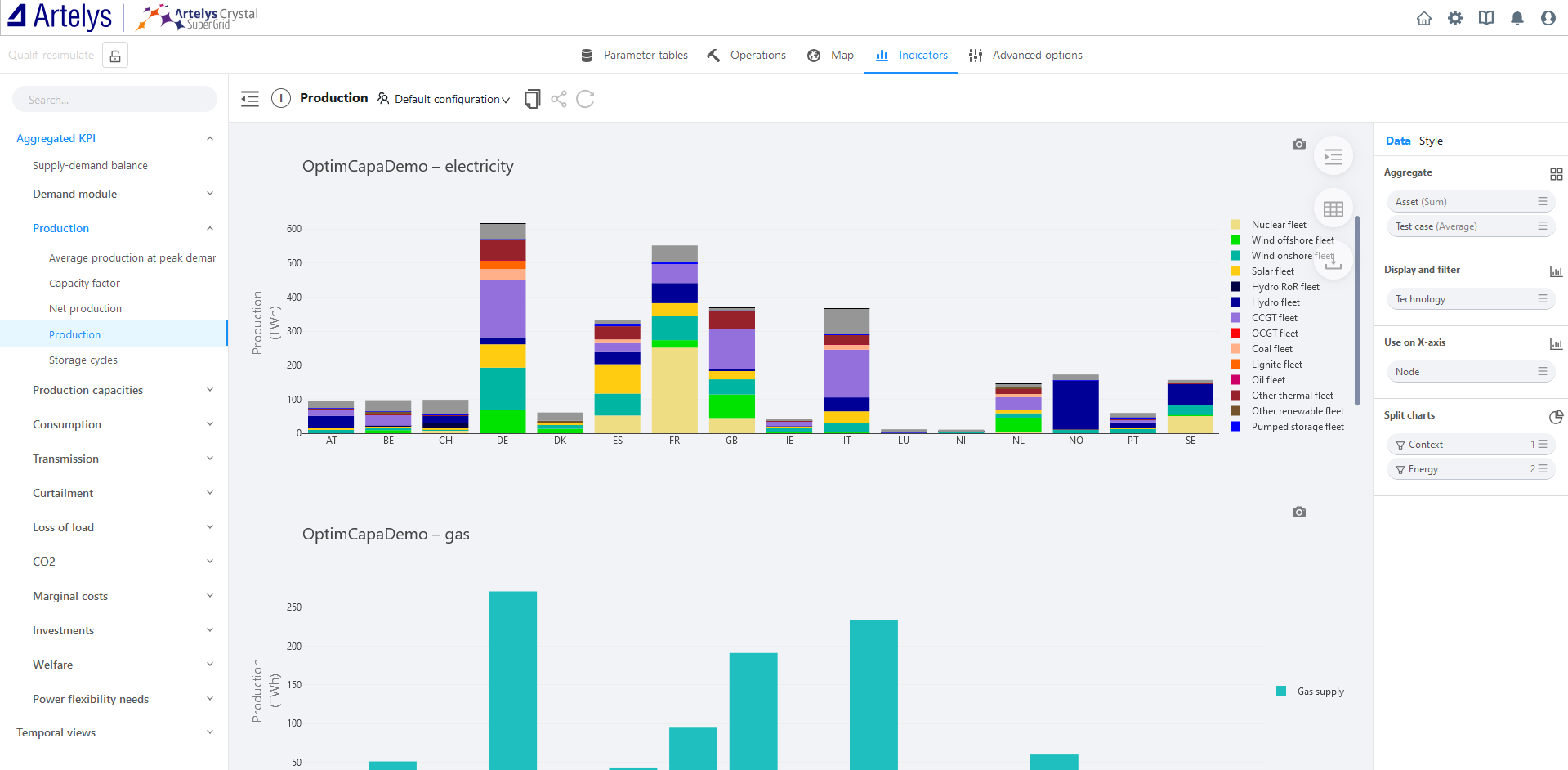
The left side of the view displays a list of all available Key Performance Indicators (KPIs). For more information about the available KPIs, please refer to the KPI documentation.

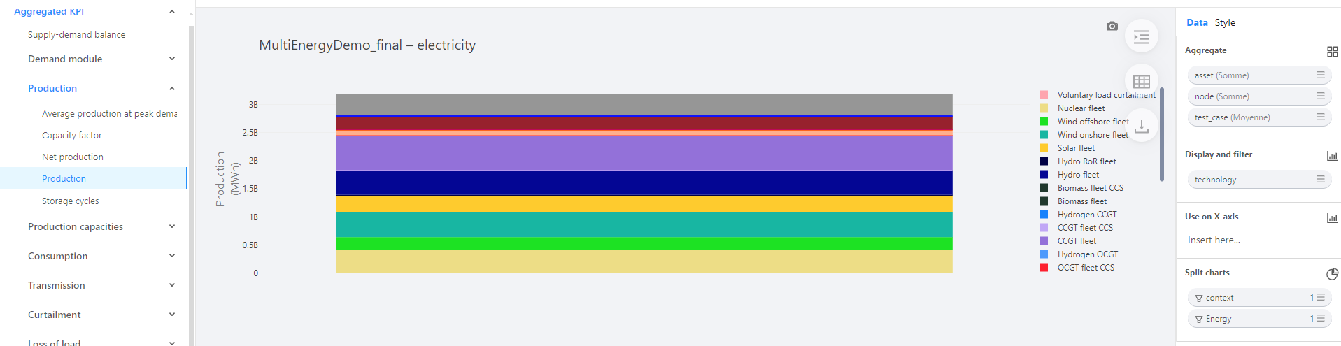
The right side of the view (under Data) allows you to configure and move the filters to create the KPI that suits your needs. For example, the KPI below shows the average electricity production over the test cases in the MultiEnergyDemo_final context, broken down by technology and aggregated by node and asset.

KPI example

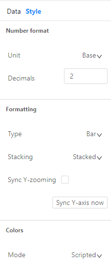
Use Style to customize the formatting, units, and colors of your KPI visualization. Select Sync Y-zooming to maintain the same Y-scale between your charts when you zoom in, facilitating easier comparison between multiple charts. The Sync Y-axis now option activates this synchronization just once, while Sync Y-zooming, keeps it active as long as you remain on this indicator.

KPI style parameters

You can save your configured KPIs using KPI configuration buttons and share your configuration with other users using Share icon .

Aggregated KPIS#

Aggregated KPIs, or Scalar KPIs, are indicators that represent totals over the entire simulation duration. Examples include total energy production (or consumption) and total CO2 emissions within the simulation timeline. These indicators can generally be aggregated (or disaggregated) by energy, context, node, test case, technology, and asset. Three types of KPI styles are available: bar (generally the default), line or pie.

Temporal views#

The Temporal views category lists Temporal KPIs. The Assets category contains temporal indicators by asset, while the Nodes category contains temporal indicators by node.

By default, the time granularity of temporal views matches the timestep duration of your context. However, you can change the time granularity of the displayed indicator by modifying the parameters under Time:

Temporal KPIs style parameters

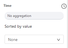
The Granularity can take the following values: Non, hour, day, week or month.
The Aggregation parameter can take the following values: None, SUM, AVG, MIN

For instance, to visualize the daily consumption trend, select the Granularity parameter day and the Aggregation parameter SUM.

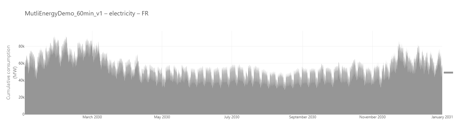
Cumulative consumption one hour granularity — Cumulative hourly consumption of electricity*

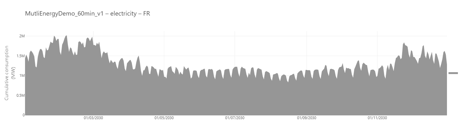
Cumulative consumption one day granularity — *Cumulative daily consumption of electricity*

Using aggregation for temporal KPIs can help to make the indicators more readable. Select the appropriate aggregation parameters according to your specific needs.

Finally, temporal views can be sorted by values in either ascending or descending order. The example below displays hourly CO2 emissions in France in the MultiEnergyDemo_60min_v1 context, sorted in descending order:

Sorted CO2 emissions in France

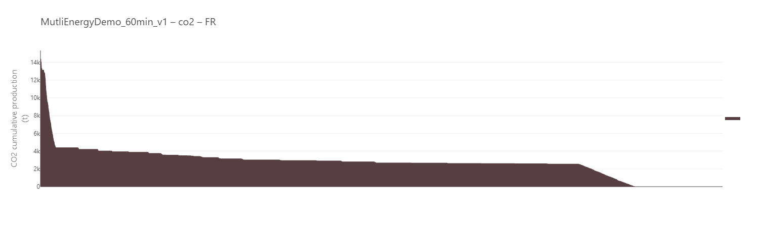
When comparing different stacked timeseries, the Ascending (synced dates) (resp. Descending (synced dates)) option sorts the series sum at each equal timestep, preserving temporal consistency. In contrast, Ascending (resp. Descending) option sorts the timeseries values independently.

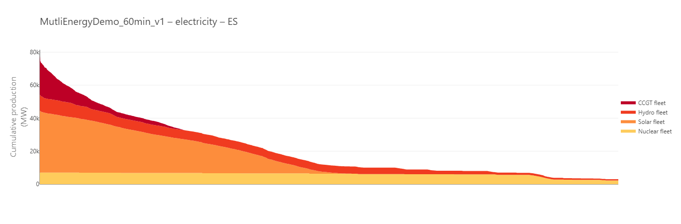
Cumulative production in Spain - no synced dates — *Cumulative production in Spain sorted by values without synchronised dates*

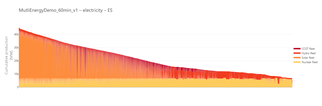
Cumulative production in Spain - synced dates — *Cumulative production in Spain sorted by values with synchronised dates*

Exporting KPIs#

When exporting KPIs, please note the following important behavior:

⚠️ Warning:

When exporting KPIs that are displayed in MW or MWh in the interface, the exported values will be in W or Wh respectively.

MW in the interface → W in the export

MWh in the interface → Wh in the export

Please adjust your calculations accordingly when working with exported data.

This conversion ensures consistency with base SI units but requires attention when interpreting the exported results.