Gas modelling

Introduction

In addition to power system simulation and optimization, Artelys Crystal Super Grid offers the ability to model and jointly optimize multi-energy systems, in order to better capture the potential synergies of sector coupling and the resulting potential reduction in total system costs. Therefore, other energy carriers such as natural gas or hydrogen, as well as the CO2 value chain, can be explicitly modelled in ACSG.

The “gas” energy stands for methane and does not distinguish natural gas from liquefied natural gas (LNG) or biogas. The modelling layer includes the different sources of gas (domestic production or imports), the European transport network and the final demands.

Gas sources

GAS PRODUCTION asset

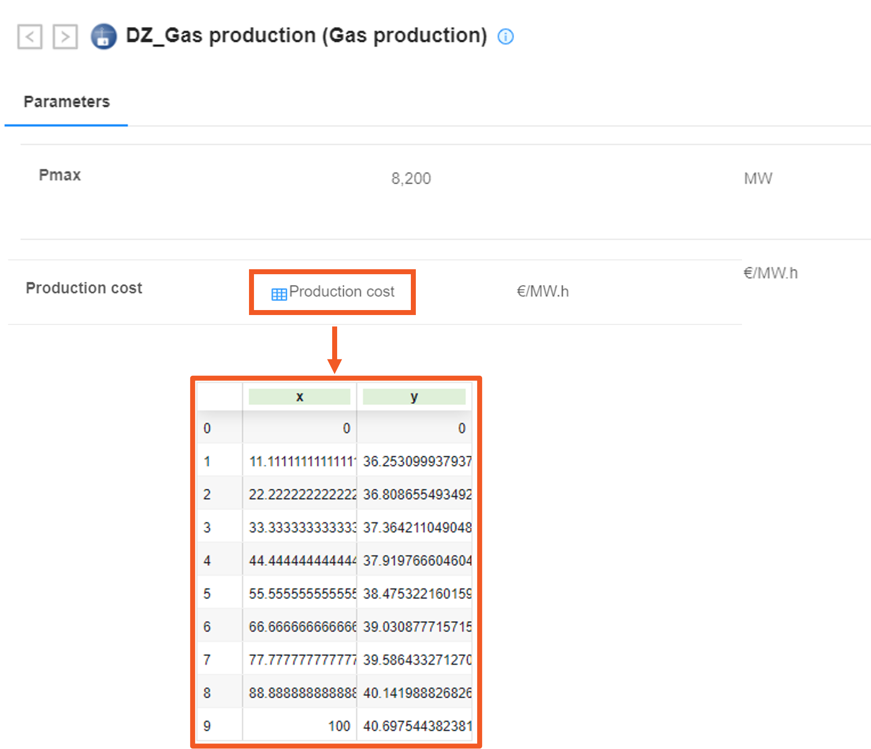
The Gas production asset is used to represent both gas production from foreign suppliers and domestic sources. It delivers gas to the connected node and includes the following key parameters:

• PMAX: This is calculated from the yearly available volumes, as gas production is empirically nearly constant;

• PRODUCTION_COST_CURVE: A cost curve which associates a cost \(y\) to a percentage of PMAX used \(x\).

This asset can be used to model:

• Domestic gas production: in this case, the MUST_RUN behavior is typically used to ensure that each country prioritizes its own domestic production.

• Foreign gas production upstream in the imports value chain: here, it is recommended to activate the GRADIENTS behavior and set the attributes GRADIENT_UP and GRADIENT_DOWN to zero. This approach enforces a constant production that is not necessarily prioritized, providing a more realistic representation of foreign gas production.

BIOGAS IMPORTS asset

The BIOGAS_IMPORTS asset represents domestic biomethane and biogas production. It supplies gas to the connected node and consumes CO2 to account for a net-zero CO2 balance for biogas used in power production: the CO2_CONSUMPTION_YIELD parameter allows to offset CO2 emissions when the produced biogas is consumed.

Since biomethane is significantly more expensive than natural gas and therefore only affordable with support mechanisms, it is recommended to prioritize it (assuming such support mechanisms are in place):

• Either by using the behavior MUST_RUN. In this case, the IMPORTS parameter represents the maximum delivered power computed from yearly available volumes.

• Either by modelling the economically attractive annual potential using the VOLUME_TARGET behavior with a supply price close to zero. This allows the model to optimize the use of biogas as a source. The STORAGE_AVAILABILITY attribute represents the maximum available annual volume.

• Or by representing explicitly the production cost of biogas (using cost curves, for example), combined with a carbon budget constraint or a sufficiently high carbon tax.

ID	Description	Behavior	Unit	Usual value
CO2_CONSUMPTION_YIELD	CO2 consumption yield w.r.t. production		t/MWh	Methane emission factor
PMAX	Pmax	Not MUST_RUN	MW
STORAGE_CAPACITY	Storage capacity	VOLUME_TARGET and not MUST_RUN	MWh	Maximum annual production volume
MINIMUM_VOLUME	Minimal target volume	VOLUME_TARGET and not MUST_RUN	MWh	Minimum annual production volume
IMPORTS	Inelastic imports (timeseries or constant value)	MUST_RUN	MW
PRODUCTION_COST_CURVE	Production cost (a constant or a cost curve)		€/MWh	Production cost (emission cost excluded)

It is also possible to avoid prioritizing biogas production if the goal is to study the need for support mechanisms.

Biogas imports - VOLUME_TARGET behavior

The behavior VOLUME_TARGET activates the following attributes:

ID	Description	Type	Unit	Usual value
STORAGE_CAPACITY	Storage capacity	Constant	MWh	Maximum annual production volume
MINIMUM_VOLUME	Minimal target volume	Constant	MWh	Minimum annual production volume
MIN_PROFILE	Minimal volume profile	Constant or timeseries	%	Minimal share of the minimum volume that must have been produced at time step \(t\)
STORAGE_AVAILABILITY	Maximal volume profile	Constant or timeseries	%	Maximal share of the storage capacity that can have been produced at time step \(t\)

At the end of the simulation, the total biogas production must be between MINIMUM_VOLUME and STORAGE_CAPACITY:

\[minVolume \leq annualProduction \leq storageCapacity\]

Profiles (percentages) are used to limit cumulative production at each time step \(t\) of the simulation:

\[minVolume * minProfile \leq cumulativeProduction_{(t)} \leq storageCapacity * storageAvailability_{(t)}\]

Example 1: To ensure that 100% of the biogas potential is used at the end of the simulation, it is necessary to:

• Set \(minProfile\) to 0 for all time steps except the last, and set the last time step to 100

• Set \(minVolume = storageCapacity\)

• Set \(storageAvailability = 100\)

Example 2: To ensure that no more than 50% of the total biogas potential is used by the end of the first quarter, set \(storageAvailability = 50\) for the entire first quarter.

Modelling gas imports

The LNG channel

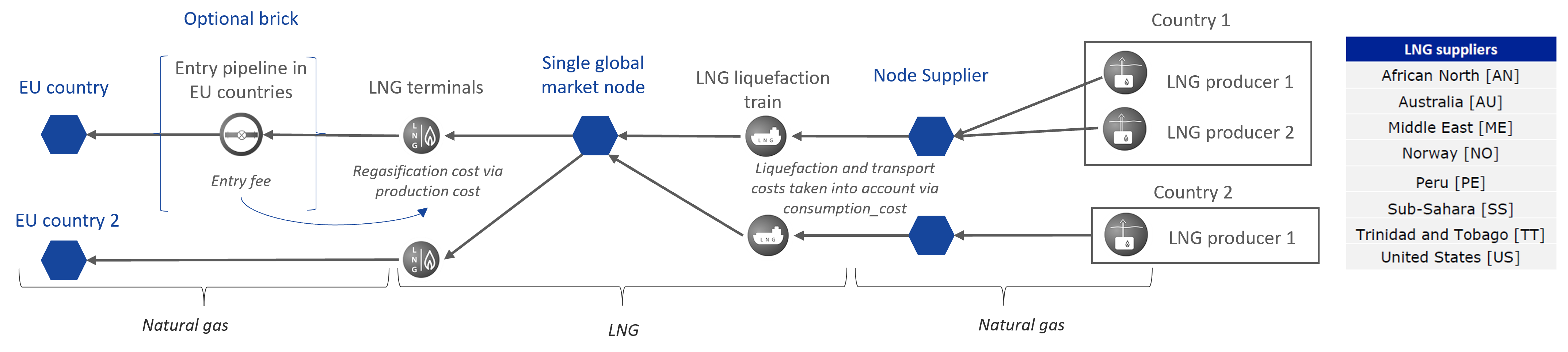
• Setting up gas production in supplier countries : the total volume available for the whole year can be defined through the \(PMAX\) attribute (\(PMAX = \frac{Volume}{8760}\)). A cost curve is defined, associating a cost \(y\) to a percentage of \(PMAX\) used \(x\). Set GRADIENT_UP = GRADIENT_DOWN = 0 to better reflect reality and represent the flexibility needs of the European gas system (see Gas production for more details).

• LNG liquefaction train : Defined with an infinite capacity to ensure no congestion occurs during shipping.

• Gas trading on the LNG market node

• EU imports via LNG terminals : EU countries can import LNG through terminals that provide unloading, storage and gasification services. There are 30 LNG terminals in Europe, 3 in Great Britain. LNG terminal assets are modeled as a combination of storage and pipeline assets. They have a certain storage capacity (set to a capacity much lower than nationals levels) but can operate in only one direction, producing gas for the importing EU country and not sending back LNG to the LNG market node.

Import pipelines

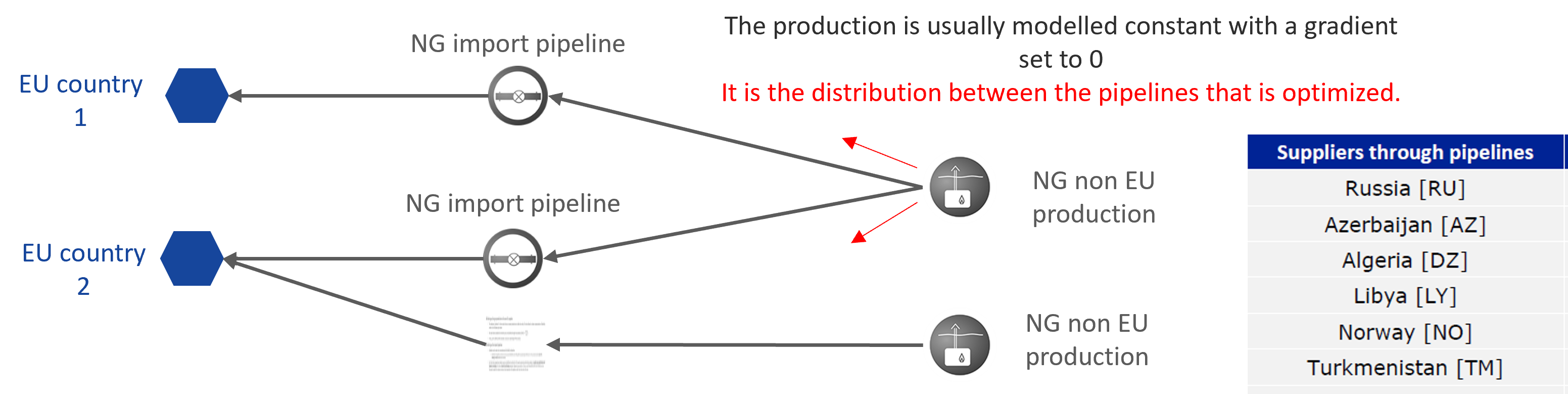
Setting up gas production in non-EU supplier countries : Refer to the LNG channel and Gas production sections.

Setting up import pipelines :

• Gradients can be used to avoid overestimating pipeline flexibility. Sometimes, the gradient can even be set to zero to impose a fixed flow on a pipeline. This can also model OTC exchange contracts between two countries.

• For short-term prospective studies, additional constraints can be set to this purely economic optimization problem to model current realities, such as long-term exchange agreements between countries. To do so, an attribute MIN_FLOW (% of PMAX) can be set on the pipeline to model the minimum volume that must be imported via this pipeline, which must be met at all costs.

The GAS_IMPORTS asset allows modeling this import chain implicitly.

Modelling gas demand

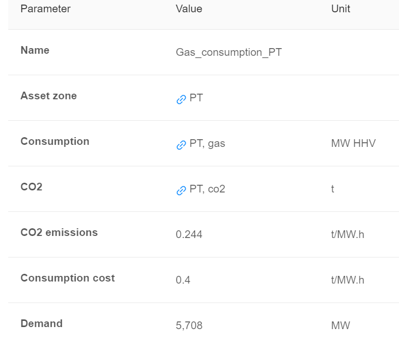
GAS CONSUMPTION asset

The GAS_CONSUMPTION asset represents an inelastic final gas demand. It accounts for all the exogenous end-uses of gas, either in the industry, transport or building sectors. This demand excludes gas-to-power usage, as it falls under optimization within the electricity layer. End-uses can be associated to hourly profiles, for instance thermosensitive or non-thermosensitive demands. This asset represents the demand for gas as an energy carrier: since the gas is burned in this case, the CO2 emissions resulting from its consumption are accounted for.

DEMAND asset

The asset DEMAND represents an inelastic demand. This asset can model various energy demands. In particular, it can be used to model a non-energy demand for gas (gas is used as a molecule). Thus, **CO2 emissions related to gas demand are not accounted for in this asset.

The DEMAND attribute can be either a timeseries or a constant.

Modelling hint

When there is a demand but no associated supply for a given energy in the node considered, add a loss of load asset for this energy on this node to avoid infeasibilities.

Gas infrastructures

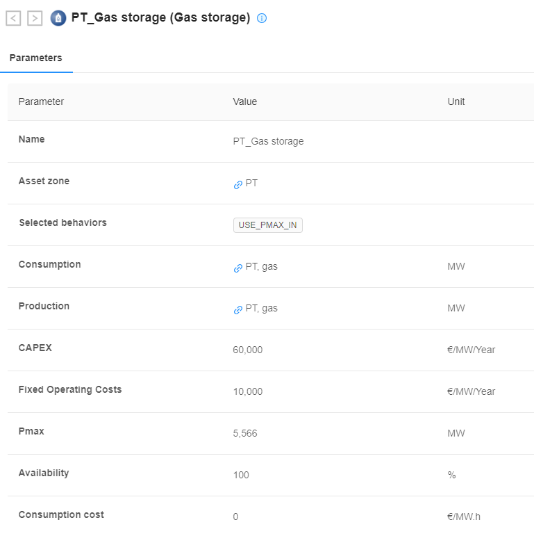
GAS_STORAGE asset

GAS_STORAGE assets can consume, store and inject gas on the national networks (NB: for some storage assets, the country filling it and the country using it may be different).

Injection and withdrawal available capacities are computed in the model by 4 attributes:

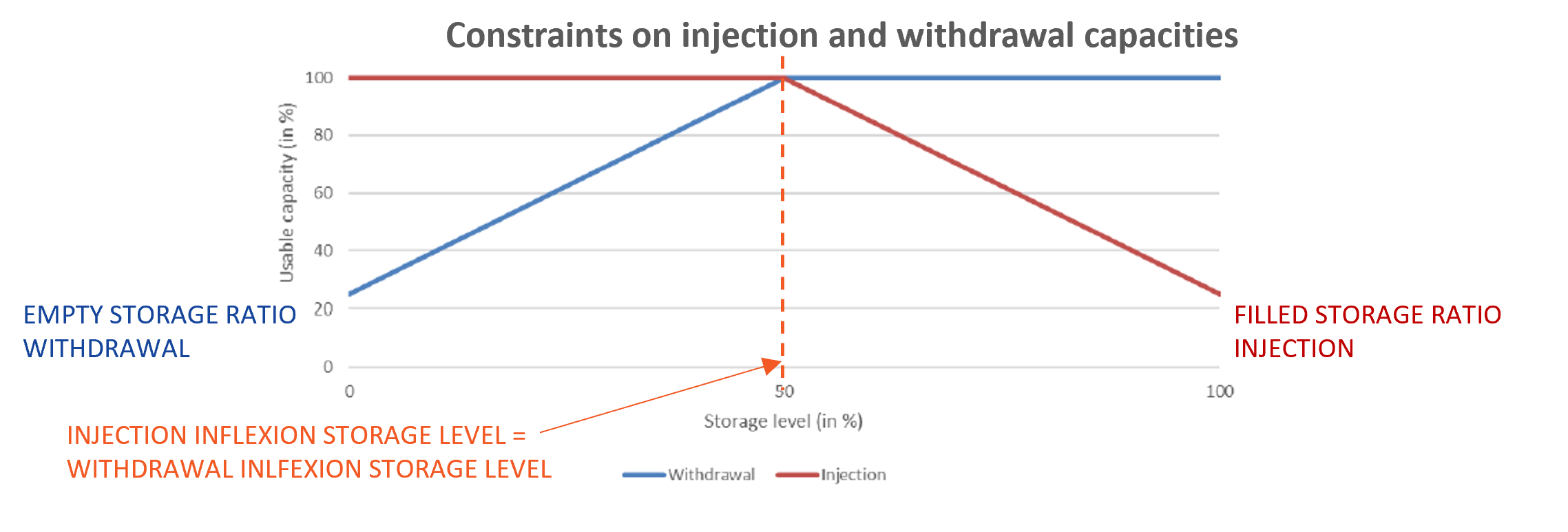
This models the increasing difficulty of compressing gas for injection as the storage becomes fuller and of withdrawing gas as the storage becomes emptier.

The storage capacity (in MWh HHV) is given by the attribute STORAGE_CAPACITY.

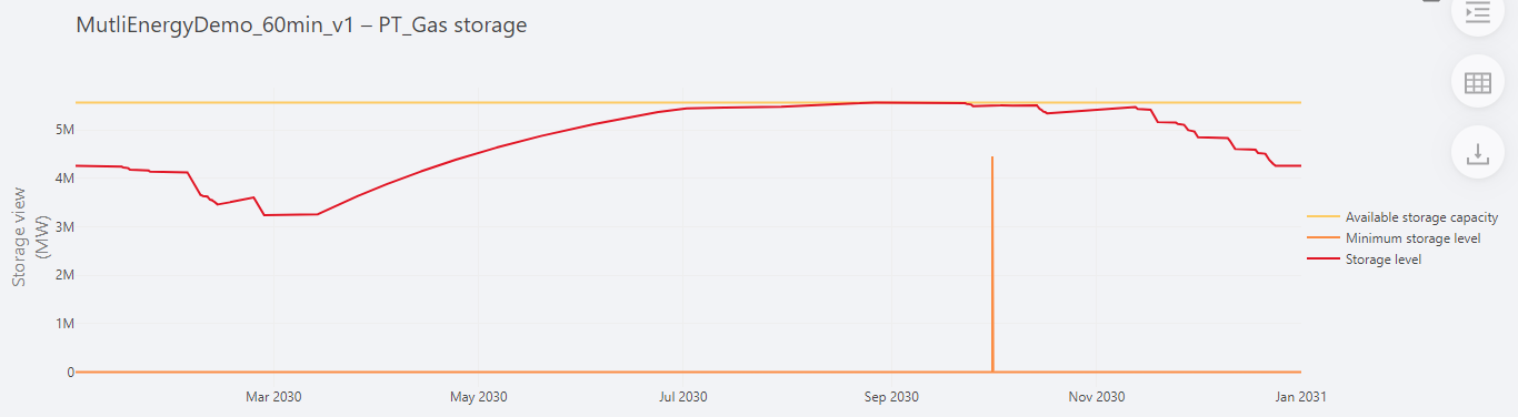
An additional constraint, defined by the MIN_STORAGE_LEVEL attribute, requires the storage to be filled to 80% by October 1st to ensure adequate supply during winter.

Gas storage assets are crucial for meeting the seasonal flexibility needs of the European gas system:

• A low demand in summer and a very high demand in winter with constant gas production throughout the year.

• Storage assets are filled during the summer and used during the winter to supplement gas imports.

Gas line packs

Gas system models typically operate on a daily basis. For instance, ENTSO-G data us usually provided in GWh/day for both production and demand.

However, the model in ACSG ensures supply-demand equilibrium at every node, at every hourly time step and for each energy type. To account for this system’s daily flexibility, the gas system model in ACSG uses a gas storage assetconfigured as follows:

• A very high PMAX and 24-hour storage capacity (using the DISCHARGE_TIMES behavior with the DISCHARGE_TIME attribute set to 24);

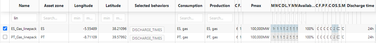
• The minimum storage level and available storage capacity are configured to ensure that every 24 hours, the storage returns to its initial level:

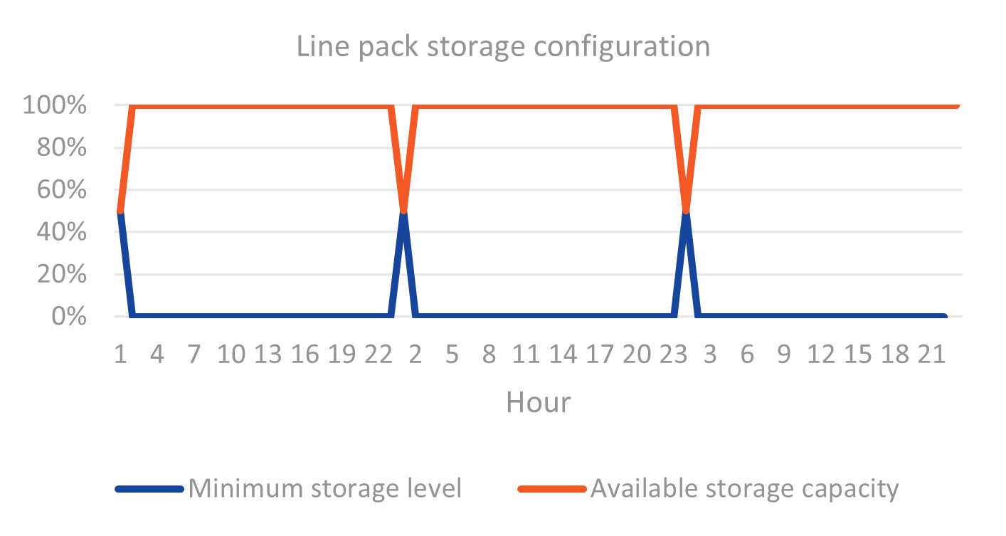
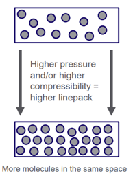
These assets are often referred to as “linepacks”. Actually, the term “linepack” refers to the ability of gas pipelines to store a certain amount of energy by adjusting the pressure differential between the input and the output. This kind of operational flexibility frees gas systems from the challenge of hourly balancing supply and demand, which must be taken into account when modeling power systems, for example.

For more information about linepack, see here.

PIPELINE asset

Gas pipelines (PIPELINE assets) allow gas exchanges between two nodes. Their capacities can be optimized, and the flow within the pipeline can be constrained using the GRADIENTS behavior.