Contribution to flexibility needs (MWh)

indexed by: asset, flexibility timescale, node, technology, test case

Description

This KPI aims to indicate the various assets that provide flexibility to the system and quantifiy the contribution of each one to answer the flexibility needs of a given node at a given flexibility timescale. These assets can be generation assets, demand assets that are capable of optimising their consumption to consume at times when demand is lower, net imports or curtailment wells (absorbing artificially production surplus). This KPI is directly in front of the KPI Flexibility needs : in fact, the assets meet directly the demand for flexibility calculated in this KPI.

This flexibility needs can be analysed over three different timescales, as in the Flexibility needs KPI : daily, weekly and annually. This helps us to understand the type of flexibility provided by an asset For instance, a smart-charging electric vehicle, optimizing his consumption, may shift his peak consumption and provide daily flexibility when a hydraulic dam may respond more to the needs for seasonal flexibility (annual timescale).

The quantification of an asset’s contribution to meeting the system’s flexibility needs is based on a comparison between variations in its optimised production/consumption and variations in residual load at the corresponding node. As a reminder, residual load corresponds to unoptimized electricity demand minus renewable energy production. At a given timescale and a given node, a technology contributed “positively” to the concerned flexibility needs if its generation increases (resp. decreases) when the residual load increases (resp. decreases) and negatively if it is the other way round.

This principle is illustrated in the figure below for daily flexibility needs.

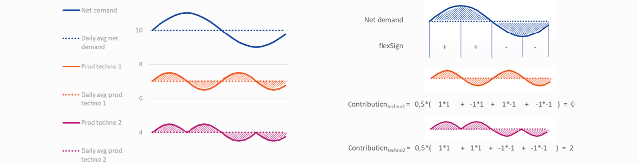
Modelling hint

For a given flexibility timescale, a given node and a given test case, the sum of all the contributions to the concerned flexibility needs are equal to the flexibility needs computed in the Flexibility needs KPI.

Calculation

The calculation of this KPI is based on the same principle that the one in the KPI Flexibility needs. All the equations below are valid for any realization and are therefore implicitly indexed by test case.

For each realization, contribution to flexibility needs for power systems are calculated based on the residual load. Let be \(y_{n}(t)\) the residual load of node \(n\). This can be express as:

\[y_{n}(t) = d_{n}(t) - \sum\limits_{a \in A_{n}^{p,RES}} p_a(t) - \sum\limits_{b \in B_{n}^{p,Hydro}} p^{*}_a(t).min\_load_a(t)\]

with \(d_{n}(t)\) the unoptimized demand of pure demand assets (storages, transmissions are not included here) at node \(n\).

As explained in the above paragraph, different types of asset can contribute to the flexibility needs. The calculation of their aggregate contribution is based on their contribution at each time step \(z(t)\).

• Pure electricity producing assets: their contribution corresponds to their production at each timestep \(z_{a,n}(t) = p_{a,n}(t)\). This concerns electricity producers only.

• Assets consuming electricity to produce another energy: their contribution corresponds to the inverse of their consumption at each timestep \(z_{a,n}(t) = p_{a,n}(t)\). Electrolysers are an example of these assets.

• Flexible demand assets: their contribution corresponds to the difference between their unoptimized demand and their optimized at each timestep \(z_{a,n}(t) = \hat{c}_{a,n}(t) - c_{a,n}(t)\) with \(\hat{c}_{a,n}(t)\) the unoptimized demand of these assets. The modeled optimized assets are electric vehicles, heat-pumps, demand-response and interruptible load.

• Storage assets: their contribution corresponds to the difference between their production and their consumption (operating point) \(z_{a,n}(t) = p_{a,n}(t) - c_{a,n}(t)\).

• Net imports: their contribution corresponds the net imports at the zone at each timestep, which is the inverse of the electric net position of the node. \(z_{a,n}(t) = - \delta_{electricity,n}(t)\) with \(\delta_{electricity,n}(t)\) the electrical net position of node \(n\). The details of net position calculation are described in the KPI Net position.

• Curtailment wells: their contribution is defined as the inverse of their consumption enabling to absorb production surplus and mostly renewable ones at each timestep \(z_{a,n}(t) = c_{a,n}(t)\). This concerns only assets \(a\) with \(a \in A_{n}^{well}\) the set of well assets consuming electricity at node \(n\).

Daily flexibility needs

The first calculation stage consist in calculating both:

• the daily-averaged residual load for the node \(n\) for each day \(\tilde{y}_{n}^{D}(t) = \langle y_{n}(t) \rangle_{t \in Day(t)}\)

• the daily-averaged contribution to flexibility needs of asset \(a\) for the \(n\) for each day \(\tilde{z}_{a,n}^{D}(t) = \langle z_{a,n}(t) \rangle_{t \in Day(t)}\)

Then the sign \(\zeta_{n}^{D}(t)\) of the variations of the residual load relatively to the daily average residual load must be computed.

\[\zeta_{n}^{D}(t) = f(y_{n}(t)-\tilde{y}_{n}^{D}(t))\]

with \(f(x) = \begin{cases} \quad -1 \text{ if} x < 0\\ \quad 0 \text{ if} x = 0\\ \quad 1 \text{ if} x > 0 \end{cases}\)

Let be \(x_{a,n,D}\) the contribution to daily flexibility needs for the asset \(a\) the node \(n\). We can then express \(x_{a,n,D}\) as :

\[x_{a,n,D} = \frac{1}{2}.\sum_t{\zeta_{n}^{D}(t)*[z_{a,n}(t)-\tilde{z}_{a,n}^{D}(t)]}\]

Weekly flexibility needs

A similar calculation is carried out in order to obtain contributions to weekly flexibility needs, only changing the timescale. First weekly-averaged residual load and contribution to flexibility needs of asset \(a\) must be computed.

• the weekly-averaged residual load for the node \(n\) for each week \(\tilde{y}_{n}^{W}(t) = \langle y_{n}(t) \rangle_{t \in Week(t)}\)

• the weekly-averaged contribution to flexibility needs of asset \(a\) for the \(n\) for each week \(\tilde{z}_{a,n}^{W}(t) = \langle z_{a,n}(t) \rangle_{t \in Week(t)}\)

Then the sign \(\zeta_{n}^{W}(t)\) is computed as \(\zeta_{n}^{W}(t) = f(\tilde{y}_{n}^{D}(t)-\tilde{y}_{n}^{W}(t))\) Therefore, the contribution to weekly flexibility needs for the asset \(a\) the node \(n\), \(x_{a,n,W}\), can be express as

\[x_{a,n,W} = \frac{1}{2}.\sum_t{\zeta_{n}^{W}(t)*[\tilde{z}_{a,n}^{D}(t)-\tilde{z}_{a,n}^{W}(t)]}\]

Annually flexibility needs

The calculation for annually flexibility needs relies on the same principle. Let’s first calculate some intermediary results.

• the monthly-averaged residual load for the node \(n\) for each month \(\tilde{y}_{n}^{M}(t) = \langle y_{n}(t) \rangle_{t \in Month(t)}\)

• the monthly-averaged contribution to flexibility needs of asset \(a\) for the \(n\) for each month \(\tilde{z}_{a,n}^{M}(t) = \langle z_{a,n}(t) \rangle_{t \in Month(t)}\)

• the yearly-averaged residual load for the node \(n\) for each year \(\tilde{y}_{n}^{A}(t) = \langle y_{n}(t) \rangle_{t \in Year(t)}\)

• the yearly-averaged contribution to flexibility needs of asset \(a\) for the \(n\) for each year \(\tilde{z}_{a,n}^{A}(t) = \langle z_{a,n}(t) \rangle_{t \in Year(t)}\)

Then the sign \(\zeta_{n}^{A}(t)\) is computed as \(\zeta_{n}^{A}(t) = f(\tilde{y}_{n}^{M}(t)-\tilde{y}_{n}^{A}(t))\)

Finally, the contribution to annually flexibility needs for the asset \(a\) the node \(n\), \(x_{a,n,A}\), can be express as

\[x_{a,n,A} = \frac{1}{2}.\sum_t{\zeta_{n}^{A}(t)*[\tilde{z}_{a,n}^{M}(t)-\tilde{z}_{a,n}^{A}(t)]}\]

For more information about the flexibility needs definition, please refer to Flexibility needs indicator.

Global variables and parameters notations definitions can be consulted here.

Indexing

• The asset and technology index refers to the name of the asset and the technology type of the asset meeting flexibility needs

• The node index of this KPI refers to the node both demand and production assets are related to for the calculation of the residual load or the contributions

• The flexibility timescale index of this KPI refers to the timescale for which flexibility needs are computed (daily, weekly or annually)

• The test case index corresponds the test case of the realization variables and parameters are taken from

• There is no energy index in this KPI because it only focuses on the electrical system