Flexibility needs (MWh)

indexed by: flexibility timescale, node, test case

Description

This KPI aims to quantify the flexibility needs of an electrical system, i.e. the i.e. the energy needs required to absorb variations in residual load (unoptimized electricity demand minus renewable generation) relative to its average. Variations in residual demand are considered here, rather than pure demand, because the focus is on the need for flexibilities, as opposed to renewables, which are not pilotable.

This flexibility needs can be analysed over three different timescales : daily, weekly and annually. This makes it possible to understand whether the necessary flexibilities need to be adapted to a daily, weekly or seasonal operation. For example, a system may have a high need for daily flexibility to absorb solar production and peak demand in the early evening, but little need for weekly/annual flexibility, assuming, for example, that there is little temperature-sensitive demand in the system, which varies according to the season.

Modelling hint

This KPI facilitates the understanding of the extent to which rising RES shares increase flexibility needs at different granularity over time.

Calculation

All the equations below are valid for any realization and are therefore implicitly indexed by test case. For each realization, flexibility needs for power systems are calculated based on the residual load. Let be \(y_{n}(t)\) the residual load of node \(n\). This can be express as:

\[y_{n}(t) = d_{n}(t) - \sum\limits_{a \in A_{n}^{p,RES}} p_a(t) - \sum\limits_{b \in B_{n}^{p,Hydro}} p^{*}_a(t).min\_load_a(t)\]

with \(d_{n}(t)\) the unoptimized demand of pure demand assets (storages, transmissions are not included here) at node \(n\).

Daily flexibility needs

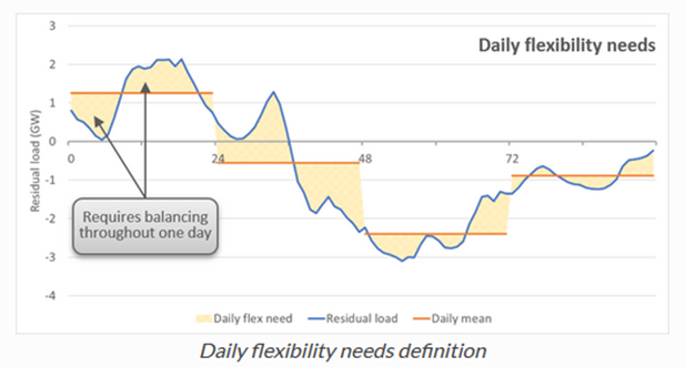
Daily flexibility needs are defined as the cumulated difference between the hourly residual load throughout a day and its daily average over the entire time horizon. The result is expressed as a volume of energy per day (e.g., GWh/day).

Summing up these daily (positive) differences over the whole simulation (365 days for a single year simulation) reveals the overall daily flexibility needs one may respond to in order to obtain a residual load that is flattened out on a daily basis.

Let be \(x_{n,D}\) the daily flexibility needs for the node \(n\). We can then express \(x_{n,D}\) as :

\[x_{n,D} = \frac{1}{2}.\sum_t{|y_{n}(t)-\tilde{y}_{n}^{D}(t)|}\]

with \(\tilde{y}_{n}^{D}(t)\) the daily-averaged residual load for the node \(n\) for each day : \(\tilde{y}_{n}^{D}(t) = \langle y_{n}(t) \rangle_{t \in Day(t)}\)

As the sum account for the absolute value of the difference between the hourly residual load throughout a day and its daily average, the factor \(\frac{1}{2}\) prevents from accounting two times the flexibility needs. The following figure shows a graphical representation of the calculation.

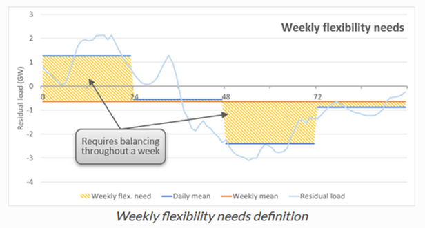
Weekly flexibility needs

A similar calculation is carried out in order to obtain weekly flexibility needs, comparing \(\tilde{y}_{n}^{D}(t)\) the daily-averaged residual load computed before (i.e., the residual load after having replied to all daily flexibility needs) with the weekly-averaged residual load \(\tilde{y}_{n}^{W}(t)\). Summing up the weekly flexibility needs of all weeks gives the overall weekly flexibility needs of the system.

This weekly-averaged residual load is defined as \(\tilde{y}_{n}^{W}(t) = \langle y_{n}(t) \rangle_{t \in Week(t)}\).

Therefore, let be \(x_{n,W}\) the weekly flexibility needs for the node \(n\). We can then express \(x_{n,W}\) as :

\[x_{n,W} = \frac{1}{2}.\sum_t{|\tilde{y}_{n}^{D}(t)-\tilde{y}_{n}^{W}(t)|}\]

Annually flexibility needs

Lastly, annually flexibility needs are calculated as the cumulated difference between the monthly-averaged residual load and the annually-averaged residual load over the entire time horizon. Let be \(x_{n,A}\) the annually flexibility needs for the node \(n\). We can then express \(x_{n,A}\) as :

\[x_{n,A} = \frac{1}{2}.\sum_t{|\tilde{y}_{n}^{M}(t)-\tilde{y}_{n}^{A}(t)|}\]

with

• The monthly-averaged residual load for the node \(n\), \(\tilde{y}_{n}^{M}(t)\), defined as : \(\tilde{y}_{n}^{M}(t) = \langle y_{n}(t) \rangle_{t \in Month(t)}\)

• The annually-averaged residual load for the node \(n\), \(\tilde{y}_{n}^{A}(t)\), defined as : \(\tilde{y}_{n}^{A}(t) = \langle y_{n}(t) \rangle_{t \in Year(t)}\)

Note

In case of dataset with temporal horizon less than one month (respectively day), annual (respectively weekly) flexibility needs will be 0.

Global variables and parameters notations definitions can be consulted here.

Indexing

• The node index of this KPI refers to the node both demand and production assets are related to for the calculation of the residual load

• The flexibility timescale index of this KPI refers to the timescale for which flexibility needs are computed (daily, weekly or annually)

• The test case index corresponds the test case of the realization variables and parameters are taken from

• There is no energy index in this KPI because it only focuses on the electrical system